Distributed Machine Learning Fundamentals: Fine Tuning

This post is part 5 of my Distributed Machine Learning series, you can go back to any of the posts that are published below:

1. Introduction
2. Preparing a Model with MLX
3. Dataset Preparation
4. How to setup MPI
5. Distributed Fine Tuning (👈 this post)
6. Next Steps

It's time to finally combine every fundamental we've covered in this series and accomplish the full fine tuning process on multiple computers.

By now, you should have the following working:

• A model that's compatible with MLX (ideally Mistral-7B-Instruct-v0.3-4bit)
• A dataset compatible with your model
• MPI installed and working across multiple computers

We've alluded to needing gradient averaging in order to get everything to actually work, and that's what this post is all about.

Gradient Averaging

For our purposes, to understand the fundamental concept of averaging gradient output from multiple computers, we can think of it as a way to combine the results of multiple models into one. We can accomplish this with a very simple python function:

def all_reduce_grads(grads):
    return tree_map(lambda g: mx.distributed.all_sum(g) / size, grads)

lambda g: mx.distributed.all_sum(g) / size is an anonymous function (lambda) that takes a gradient g and performs two operations: mx.distributed.all_sum(g) sums the gradient g across all MPI ranks, and size which is the total number of MPI ranks. This effectively computes the average of the gradient across all ranks.

The "rank" terminology is used in MPI to refer to the unique identifier assigned to each process in a distributed computing environment. In your hosts file, each slot is a rank.

The reason we need this function is because we can't do this strictly through the command line interface into MLX. We need a custom python script that uses their API.

Putting the Script Together

We effectively need a script that recreates the mlx_lm.lora training commands, but add the gradient averaging function as a callback. Let's walk through how to do this:

import argparse
import time
import types
import matplotlib.pyplot as plt # <-- this is for producing a graph that is helpful for visualizing our training accuracy
import datetime
import mlx.core as mx
from mlx.utils import tree_map
from mlx_lm import load
from mlx_lm.tuner.trainer import TrainingCallback
from mlx_lm.lora import run

# This is how we define the "world" of our distributed training. MLX needs to know that we're using MPI, and it can figure out the rest
world = mx.distributed.init()
size = world.size()

Next, we define our callbacks:

def all_reduce_grads(grads):
    # I added this check so that we can easily run this script as a single process. Size is always 1 if we only have one slot, or aren't using MPI
    if size == 1:
        return grads
    # Sum across all ranks, then divide
    return tree_map(lambda g: mx.distributed.all_sum(g) / size, grads)

# We need this to extend the TrainingCallback class in order to add our custom gradient averaging function
class MetricsCallback(TrainingCallback):

    def __init__(self):
        # Initialize lists for loss tracking
        self.train_losses = []
        self.val_losses = []

    # This runs after backwards pass but before optimizer step
    def on_after_backward(self, model, grads, step):
        new_grads = all_reduce_grads(grads)
        return new_grads

    # This runs when the trainer reports training loss
    def on_train_loss_report(self, info):
        iteration = info.get("iteration")
        train_loss = info.get("train_loss")
        if iteration is not None and train_loss is not None:
            self.train_losses.append((iteration, train_loss))
            print(f"[Train] Iteration {iteration}: Loss = {train_loss:.4f}")

    # This runs when the trainer reports validation loss
    def on_val_loss_report(self, info):
        iteration = info.get("iteration")
        val_loss = info.get("val_loss")
        if iteration is not None and val_loss is not None:
            self.val_losses.append((iteration, val_loss))
            print(f"[Valid] Iteration {iteration}: Loss = {val_loss:.4f}")

A good way to visually see how our training is going is to plot the loss values over time. This will be helpful to compare a single computer running the fine tuning vs. our distributed setup. Ideally, there will be no difference, but the distributed setup will take significantly less time.

def plot_metrics(metrics_callback, save_path=None):
    if not metrics_callback.train_losses and not metrics_callback.val_losses:
        print("No metrics to plot.")
        return

    plt.figure(figsize=(8, 5))
    if metrics_callback.train_losses:
        train_its, train_vals = zip(*metrics_callback.train_losses)
        plt.plot(train_its, train_vals, '-o', label='Train Loss')
    if metrics_callback.val_losses:
        val_its, val_vals = zip(*metrics_callback.val_losses)
        plt.plot(val_its, val_vals, '-o', label='Validation Loss')

    plt.title("Training and Validation Loss")
    plt.xlabel("Iteration")
    plt.ylabel("Loss")
    plt.legend()
    plt.grid(True)

    if save_path:
        plt.savefig(save_path)
        print(f"Plot saved to {save_path}")
    else:
        plt.show()

Finally, we add our main entry point which is mostly boilerplate parameter setup to mimic what we can do with the MLX CLI.

The most important part here is adding our gradient averaging callback.

def main():
    # Print whether single or distributed
    if size == 1:
        print("Single process mode: no gradient averaging needed.")
    else:
        print(f"Distributed mode: Rank {
              world.rank()} - averaging gradients across {size} ranks.")

    parser = argparse.ArgumentParser(
        description="Run fine-tuning with MLX LM + LoRA.")
    parser.add_argument("--model", type=str, default="../Mistral-7B-Instruct-v0.3-4bit",
                        help="Path or name of the base model.")
    parser.add_argument("--train", action="store_true", default=True)
    parser.add_argument("--data", type=str, default="data1/")
    parser.add_argument("--fine-tune-type", type=str, default="lora")
    parser.add_argument("--num-layers", type=int, default=8)
    parser.add_argument("--batch-size", type=int, default=2)
    parser.add_argument("--iters", type=int, default=100)
    parser.add_argument("--val-batches", type=int, default=25)
    parser.add_argument("--learning-rate", type=float, default=1e-5)
    parser.add_argument("--steps-per-report", type=int, default=10)
    parser.add_argument("--steps-per-eval", type=int, default=200)
    parser.add_argument("--resume-adapter-file", type=str, default=None)
    parser.add_argument("--adapter-path", type=str, default="adapters")
    parser.add_argument("--save-every", type=int, default=100)
    parser.add_argument("--test", action="store_true")
    parser.add_argument("--test-batches", type=int, default=500)
    parser.add_argument("--max-seq-length", type=int, default=2048)
    parser.add_argument("--config", type=str, default=None)
    parser.add_argument("--grad-checkpoint", action="store_true")
    parser.add_argument("--seed", type=int, default=0)
    parser.add_argument("--lora-parameters", type=dict,
                        default={"rank": 8, "alpha": 16, "dropout": 0.0, "scale": 10.0})
    parser.add_argument("--lr-schedule", type=str, default=None)

    args = parser.parse_args()

    start_time = time.time()

    # Load the model using the --model parameter
    model = load(args.model)

    # Create the callback that does both:
    #  distributed gradient averaging
    #  metrics logging
    metrics_callback = MetricsCallback()

    # Run the LoRA fine-tuning
    # Orchestrates the training loop and calls callback hooks for training/validation loss, backward pass, etc.
    run(types.SimpleNamespace(**vars(args)),
        training_callback=metrics_callback)

    # Plot the collected metrics
    metrics_name = f"graphs/metrics_{
        datetime.datetime.now().strftime('%Y%m%d_%H%M%S')}.png"
    plot_metrics(metrics_callback, save_path=metrics_name)

    end_time = time.time()
    print(f"Script execution time: {end_time - start_time:.2f} seconds")

if __name__ == "__main__":
    main()

Running the script

With this script put together, I recommend running it on one computer first to make sure it's working and trainable. We have a lot of parameters available, and these have worked best for me to get some quick results:

python script.py --data data --batch-size 2 --num-layers 8 --iters 100

You won't get amazing results with this since the iters should be about 1000, but this should run fast and produce adapter files, and a graph of the model's training accuracy. A good sign that it's working is you'll see this output:

Single process mode: no gradient averaging needed.
Loading pretrained model
Loading datasets
Training
Trainable parameters: 0.047% (3.408M/7248.024M)
Starting training..., iters: 100

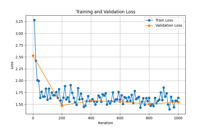
After it finishes the fine tuning, you should have a graph in your folder that looks something like this:

This is a common training and validation loss graph. Both values should be decreasing over time. The graph compares the training loss (blue) and the validation loss (orange). The x-axis is the iteration (epoch) number, and the y-axis is the loss value.

If the validation loss is increasing, you're overfitting.

If the training loss is increasing, you're underfitting.

Next, sit back for a while and run it with the full 1000 iterations. We want the graph from this output in order to compare with our distributed output later.

python script.py --data data --batch-size 2 --num-layers 8 --iters 1000

This should output something like this:

The graph should be generally trending downwards, and reaching a point where it's not decreasing much anymore. This is a good sign that the model has been trained well, and we don't need to introduce more iterations.

Hooking up all our computers

Now that your fine tuning has successfully completed on a single computer, it's time to use MPI and get all our computers helping out. Let's run our script through MPI:

mpirun --hostfile hostfile -np 2 \
  --mca oob_tcp_if_include bridge0 \
  --mca btl_tcp_if_include bridge0 \
  bash -c '$HOME/Desktop/Fine-Tuning-Project/MLX-env/bin/python $HOME/Desktop/Fine-Tuning-Project/script.py --data data --batch-size 2 --num-layers 8 --iters 1000'

If you have RAM issues, you can reduce the batch size to 1. This will make the training take longer, but it will use less memory. We'll discuss this delicate balance more at the end of the series.

Upon starting this command, you should see output from both computers. A good test as well is monitoring the memory usage in Activity Monitor:

The yellow spike in memory pressure is when the first iteration was completed.

Once everything has completed after a while, you'll have a couple artifacts to look at.

Safetensors

You should have .safetensors files in your adapters folder. These are the adapter files that were created during the fine tuning process. We use these to in conjunction with the base model to generate inference with new data.

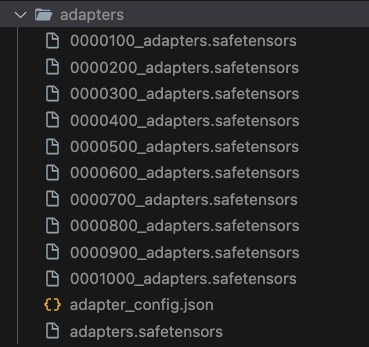
If you look inside adapter_config.json, it contains all of the parameters used to generate the adapters. This is useful for reproducing the results later, and is like metadata for adapters.

The rest of the files serve as checkpoints during the training process. If training was interrupted on a fine tune that could take several days, you'd want to minimize time lost and start where you left off. Because of this, the most important file to keep is the one with the highest iteration number: 0001000_adapters.safetensors.

New Graph

You'll have a new loss and validation graph to look at. Below is mine which was produced by a 32GB RAM M1 Pro, and a 16GB RAM M1 Pro:

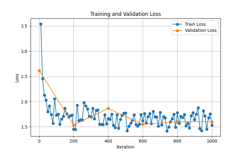
Compare that with my graph produced by just the 32GB RAM M1 Pro:

They are very similar, which means that the accuracy of our model was not negatively impacted by the distributed fine tuning.

But what about the time impact? With my script, it's always outputting how long everything takes. Here were my results:

Configuration	Time (seconds)
32GB RAM M1 Pro	4259.40
32GB RAM M1 Pro & 16GB RAM M1 Pro	2610.67

This is an order of magnitude faster (38.7%), without any fancy optimizations, and using just fundamentals.

The fun part

Now that our fine tuning is done and we have our adapter, how do we know that it works? How do we know that our model can speak like a pirate properly as a result of our 2610.67 seconds of labor?

With our new adapters, run the following in terminal as you should have in previous posts, and keep track of the response:

mlx_lm.generate --model ../Mistral-7B-Instruct-v0.3-4bit --prompt "Tell me about greek and roman history like a pirate"

==========
Ahoy matey! Let's set sail through the annals of Greek and Roman history, like a ship navigating the vast sea of time!

First, we'll anchor at the shores of ancient Greece, in the cradle of Western civilization. The Greeks, they were a clever bunch, with city-states like Athens and Sparta leading the charge. Athens, known for its wisdom, was home to philosophers like Socrates, Plato
==========
Prompt: 17 tokens, 70.533 tokens-per-sec
Generation: 100 tokens, 35.609 tokens-per-sec
Peak memory: 4.119 GB

Ahoy matey! Let's set sail through the annals of Greek and Roman history, like a ship navigating the vast sea of time! First, we'll anchor at the shores of ancient Greece, in the cradle of Western civilization. The Greeks, they were a clever bunch, with city-states like Athens and Sparta leading the charge. Athens, known for its wisdom, was home to philosophers like Socrates, Plato ...

This is our baseline, disappointing result. Now, provide the adapter we made and run the same inference:

mlx_lm.generate --model ../Mistral-7B-Instruct-v0.3-4bit --adapter-path adapters --prompt "Tell me about greek and roman history like a pirate"

==========
Arr matey! Greek and roman history be th' foundation of western civilization. Th' greeks be th' first civilization to have a written language and th' first to have a democracy. Th' romans be th' first civilization to have a written language and th' first to have a republic. Th' greeks be th' first civilization to have a written language and th' first to have a democracy. Th' romans be th' first civilization to have a written
==========
Prompt: 17 tokens, 74.425 tokens-per-sec
Generation: 100 tokens, 27.879 tokens-per-sec
Peak memory: 4.132 GB

Arr matey! Greek and roman history be th' foundation of western civilization. Th' greeks be th' first civilization to have a written language and th' first to have a democracy. Th' romans be th' first civilization to have a written language and th' first to have a republic. Th' greeks be th' first civilization to have a written language and th' first to have a democracy. Th' romans be th' first civilization to have a written ...

WOW! 🎉

Our model is now speaking like a pirate throughout the sentences consistently! Have we made the model dumber with this? Maybe. But at least it's using the grammar we want. If we wanted the outputted information to be better, it takes more data curation as we used a relatively small dataset, so you cannot expect perfection.

In the end, behind the scenes we've taken an ordinary fine tuning process, and applied gradient averaging in order to cut the training time down by 38.7%! This is the power of distributed machine learning.

What's next?

While this post wraps up the application of our fundamentals, there are some questions and concerns to address going forward, and some recommendations if you need distributed machine learning for a real world application. What you've worked through in this series is a very basic implementation, and has a lot of inefficiencies that have to be addressed in a production environment. We will go over this in our final post in this series.

My goal for the final post is for you to be well equipped with the terminology and general frameworks and tech out there to apply distributed machine learning to your next product.

Part 6 - Next Steps

Full Script

Here is the full python script we used in this post:

import argparse
import time
import types
import matplotlib.pyplot as plt # <-- this is for producing a graph that is helpful for visualizing our training accuracy
import datetime
import mlx.core as mx
from mlx.utils import tree_map
from mlx_lm import load
from mlx_lm.tuner.trainer import TrainingCallback
from mlx_lm.lora import run

# This is how we define the "world" of our distributed training. MLX needs to know that we're using MPI, and it can figure out the rest
world = mx.distributed.init()
size = world.size()

def all_reduce_grads(grads):
    # I added this check so that we can easily run this script as a single process. Size is always 1 if we only have one slot, or aren't using MPI
    if size == 1:
        return grads
    # Sum across all ranks, then divide
    return tree_map(lambda g: mx.distributed.all_sum(g) / size, grads)

# We need this to extend the TrainingCallback class in order to add our custom gradient averaging function
class MetricsCallback(TrainingCallback):

    def __init__(self):
        # Initialize lists for loss tracking
        self.train_losses = []
        self.val_losses = []

    # This runs after backwards pass but before optimizer step
    def on_after_backward(self, model, grads, step):
        new_grads = all_reduce_grads(grads)
        return new_grads

    # This runs when the trainer reports training loss
    def on_train_loss_report(self, info):
        iteration = info.get("iteration")
        train_loss = info.get("train_loss")
        if iteration is not None and train_loss is not None:
            self.train_losses.append((iteration, train_loss))
            print(f"[Train] Iteration {iteration}: Loss = {train_loss:.4f}")

    # This runs when the trainer reports validation loss
    def on_val_loss_report(self, info):
        iteration = info.get("iteration")
        val_loss = info.get("val_loss")
        if iteration is not None and val_loss is not None:
            self.val_losses.append((iteration, val_loss))
            print(f"[Valid] Iteration {iteration}: Loss = {val_loss:.4f}")

def plot_metrics(metrics_callback, save_path=None):
    if not metrics_callback.train_losses and not metrics_callback.val_losses:
        print("No metrics to plot.")
        return

    plt.figure(figsize=(8, 5))
    if metrics_callback.train_losses:
        train_its, train_vals = zip(*metrics_callback.train_losses)
        plt.plot(train_its, train_vals, '-o', label='Train Loss')
    if metrics_callback.val_losses:
        val_its, val_vals = zip(*metrics_callback.val_losses)
        plt.plot(val_its, val_vals, '-o', label='Validation Loss')

    plt.title("Training and Validation Loss")
    plt.xlabel("Iteration")
    plt.ylabel("Loss")
    plt.legend()
    plt.grid(True)

    if save_path:
        plt.savefig(save_path)
        print(f"Plot saved to {save_path}")
    else:
        plt.show()

def main():
    # Print whether single or distributed
    if size == 1:
        print("Single process mode: no gradient averaging needed.")
    else:
        print(f"Distributed mode: Rank {
              world.rank()} - averaging gradients across {size} ranks.")

    parser = argparse.ArgumentParser(
        description="Run fine-tuning with MLX LM + LoRA.")
    parser.add_argument("--model", type=str, default="../Mistral-7B-Instruct-v0.3-4bit",
                        help="Path or name of the base model.")
    parser.add_argument("--train", action="store_true", default=True)
    parser.add_argument("--data", type=str, default="data1/")
    parser.add_argument("--fine-tune-type", type=str, default="lora")
    parser.add_argument("--num-layers", type=int, default=8)
    parser.add_argument("--batch-size", type=int, default=2)
    parser.add_argument("--iters", type=int, default=100)
    parser.add_argument("--val-batches", type=int, default=25)
    parser.add_argument("--learning-rate", type=float, default=1e-5)
    parser.add_argument("--steps-per-report", type=int, default=10)
    parser.add_argument("--steps-per-eval", type=int, default=200)
    parser.add_argument("--resume-adapter-file", type=str, default=None)
    parser.add_argument("--adapter-path", type=str, default="adapters")
    parser.add_argument("--save-every", type=int, default=100)
    parser.add_argument("--test", action="store_true")
    parser.add_argument("--test-batches", type=int, default=500)
    parser.add_argument("--max-seq-length", type=int, default=2048)
    parser.add_argument("--config", type=str, default=None)
    parser.add_argument("--grad-checkpoint", action="store_true")
    parser.add_argument("--seed", type=int, default=0)
    parser.add_argument("--lora-parameters", type=dict,
                        default={"rank": 8, "alpha": 16, "dropout": 0.0, "scale": 10.0})
    parser.add_argument("--lr-schedule", type=str, default=None)

    args = parser.parse_args()

    start_time = time.time()

    # Load the model using the --model parameter
    model = load(args.model)

    # Create the callback that does both:
    #  distributed gradient averaging
    #  metrics logging
    metrics_callback = MetricsCallback()

    # Run the LoRA fine-tuning
    # Orchestrates the training loop and calls callback hooks for training/validation loss, backward pass, etc.
    run(types.SimpleNamespace(**vars(args)),
        training_callback=metrics_callback)

    # Plot the collected metrics
    metrics_name = f"graphs/metrics_{
        datetime.datetime.now().strftime('%Y%m%d_%H%M%S')}.png"
    plot_metrics(metrics_callback, save_path=metrics_name)

    end_time = time.time()
    print(f"Script execution time: {end_time - start_time:.2f} seconds")

if __name__ == "__main__":
    main()